Introduction
Under the scope of EPFL’s ADA class project, we will perform a creative extension on the paper Linguistic Harbingers of Betrayal. In this project we will work on Natural Language Processing (NLP) and more specially on Linguistic cues. As we will present to you in the next section, the authors of the paper worked on the messages of the diplomacy game and extracted some features to do some analysis and then train a simple model to perform a complex task, even for humans, which is detecting betrayal. To extend this work we will first try to train more complex and adapted models for this kind of tasks, like RNNs to see how they perform and draw some conclusions from the results. Then we will extend this work to another and completely different dataset, a dataset of news. The goal is to try and see if the same features can be used for various NLP examples.
Related Work: The Linguistic Harbingers of Betrayal paper
Since our work consists of a creative extension for the Linguistic Harbingers of Betrayal paper, we will describe briefly the work done by the authors to put you in the contest.
The authors worked on the diplomacy game, which is a war-themed strategy game where friendships and betrayals are orchestrated primarily through language. They collected a dataset, that contains 500 games half of them for games that end with an attack and the other half for games without attacks. Each game contains multiple seasons, and in each season the players communicate via messages then perform and action simultaneously. The two sets are matched to get the most accurate results. They consider an attacker the first player that breaks the friendship. For games without an attack, the attacker is chosen randomly from the two players. They performed some preprocessing to extract the following features from the messages: sentiments (negative, positive, neutral), politeness, talkativeness, discourse markers (planning, comparison, expansion, contingency, subjectivity, premises, claims). After extracting these features, they generated some plots to see and compare the behaviors of those between the two types of players. After some analysis, they fed these features to a Logistic regression model that achieved a 57% cross-validation accuracy at detecting betrayals. They concluded that the classifier can exploit subtle linguistic signals that surface in the conversation. They also analyzed how these features evolve as we get closer to betrayal to detect imbalances and check how effective the features are at detecting long-term betrayals.
Data collection
As we described in the Introduction, our project consists of two parts each of them working on a different dataset.
Diplomacy dataset
The first dataset is the Diplomacy game dataset that was provided with the paper. It contains 500 games, each game is a dictionary with 5 entries:
- seasons: a list of the game seasons
- game: unique identifier of the game it comes from
- betrayal: a Boolean indicating if the relationship ended in betrayal or not
- idx: unique identifier of the dataset entry
- people: the countries played by the players
The season entry is a dictionary with 3 entries:
- season: a year that gives you a notion of order within the seasons
- interaction: a dictionary that indicates what actions did the betrayer and victim do to each other respectively. Actions available could be either attack, support or None.
- messages: contains all the features that the authors of the “Linguistic harbingers of betrayal” rely on to analyze the messages.
The features are the following:
- sentiment: it contains the values for the positive, negative and neutral sentiments
-
lexicon_words: contains multiple entries:
allsubj: words to compute the subjectivity feature
premise: words to compute the premise feature
claim: words to compute the claim feature
disc_expansion: words to compute the expansion feature
disc_comparison: words to compute the comparison feature
disc_temporal_future: words to compute the planning feature
disc_temporal_rest: words to compute the temporal feature
disc_contingency: words to compute the contingency feature - n_requests: contains the number of requests
- frequent_words: the frequent words
- n_word’: contains the number of words
- politeness: contains the politeness of the message
- n_sentences: contains the number of sentences
According to paper, the talkativeness is quantified with the number of messages sent, the average number of sentences per message, and the average number of words per sentence.
Real and fake news dataset
The second dataset is the Fake and real news dataset (https://www.kaggle.com/clmentbisaillon/fake-and-real-news-dataset).
This dataset contains two sets, a set of Real news and another one of Fake news. Both sets contain the same features, which are:
- text: The actual text of the news article.
- title: The title of the article.
- subject: Every article is classified in a type of subject either ‘Government News’ or ‘Middle-east’ or ‘News’ or ‘US_News’ or ‘left-news’ or ‘politics’ or ‘politicsNews’ or ‘worldnews’.
- date: date of publication of the article.
The truthful articles were obtained by crawling articles from Reuters.com (News website). As for the Fake news articles, they were collected from different sources. The Fake news articles were collected from unreliable websites that were flagged by PolitiFact (a fact-checking organization in the USA) and Wikipedia. The dataset contains different types of articles on different topics, however, the majority of articles focus on political and World news topics.
Diplomacy Game:
The first part of our project consists of running an RNN model on the features extracted by the authors and test its performance. The goal of our analysis here is to see if analysis using time series can help improve the performance of the model made by the authors.
To make our model comparable to the one of the authors we try to use the same dataset and same conventions they used.
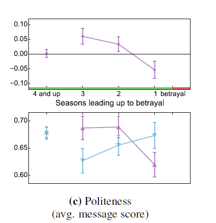
The goal of this RNN is to see if the variation of the features between the seasons has an effect on our predictive power. For example, the evolution of politeness between seasons can be quite meaningful, in fact we notice from this plot of the authors the imbalance in the politeness of the players as we get closer to betrayal.
As a first step, we extracted the average value per season for each of the features for the victims and betrayers in betrayal games. We created a dataframe containing all the features along with a label to distinguish the two players. We normalized the dataset using the z-score.
Not all games have the same number of seasons, and since the RNN model requires inputs (in our case the games) of the same size, we will pad the games with empty seasons to have all games with the same length, which is the length of the longest game in our dataset. Now all the games have 10 seasons.
RNN architecture
Our RNN model is built as follows:
- A first simple RNN layer with 10 time steps each taking a 15 dimension vector and outputting a 4 dimensions vector
- A sigmoid layer (equivalent to logistic regression) to output the prediction, regularized by elastic net
- We compile the model using the MSE loss function, the Adam optimizer and the accuracy as a metric.
- we define an early stopping to stop training if the accuracy metric has stopped improving.
We used 90% of the data for training and 10% for testing.
We show here the evolution of the binary accuracy and loss per epoch.
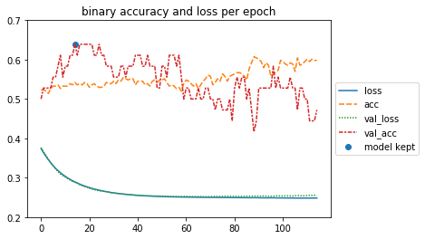
The model reached an Accuracy of 0.64 on the validation set and an accuracy of 0.55 on the test set. Which is an improvement compared to the authors’ results who only got a 0.57 cross-validation accuracy on the validation set. We also decided to test our model on non-betrayal games to see how well it performs at detecting the non-intention of betrayal. We preprocessed the non-betrayal dataset the same way as we did with the betrayal one and then we evaluated the model on it. The model reached an Accuracy of 0.58 on this test set. Thus harnessing the time evolution of the features can be helpful to the model.
However, the model has a lot of trouble converging. We don’t have a lot of data, thus to reach convergence we simplify the model as much as we can, we add batch normalization, and regularize quite heavily (high L2 values, early stopping …). Yet the problem is really complex, thus this simple model cannot fully grasp the decision boundary between betrayal or not for a given time series.
Conclusion
We want to perform more exhaustive NLP analysis with a larger dataset, to see if the NLP analysis model proposed by the authors and extended by our work generalizes well to other analogous cases.
Thus, we will now move to our new dataset to explore the effect of the linguistic cues on detecting True and Fake news.
True and Fake news:
In this second part of our project, we will deal with the True and Fake news dataset, we present to you here the different steps that we performed.
Preprocessing
The news datasets requires some preprocessing before the analysis. In fact, the news contain a lot of links, tags … that are useless for the linguistic cues analysis thus we delete them. We also map all the news to lower case letters to avoid miss-leading the models. We perform some specific modifications to remove empty strings, multiple spaces… to ensure that we have proper entries both for the analysis and the models.
Extracting features
Sentiments
coreNLP
The goal was to reproduce the same sentiment analysis as the ones done in the paper. The authors relied on the Stanford sentiment analyzer for this task. In the first part of this task we implemented methods to compute the sentiments using the Stanford coreNLP, however these computations appeared to be very time consuming ( it will take more than 2 days for the Fake news dataset only), and since we have very limited time and also limited hardware resources, we decided to limit these calculations to a subset of the datasets to see their behavior on average.
The coreNLP sentiment analyzer computes the sentiments based on how words compose the meaning of longer phrases and not on words independently. We computed the sentiments of each sentence using it and then took the average of the sentences sentiments to get the sentiments of a given news. This was performed on 3000 Real and Fake news respectively. Since the news are independent, (we estimate that 3000 is quite representative sample of the entire dataset).
We show here the average number of Sentiments with coreNLP for 3000 Fake and Real news respectively:
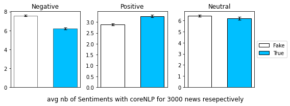
The Fake news have on average more negative sentiments but less positive sentiments than the True news for the samples that we considered. However the number of neutral sentiments seems to be close for both types. The standrad deviations are very small. We performed a statistical test to compare the mean values for the neutral sentiments but we didn’t find a significant p_value thus we cannot conclude on the difference.
TextBlob
After some research, we found that other methods exist to perform sentiment analysis, but they are usually considered less efficient than the Stanford methods, which explains the choice of the authors. This alternative method is part of the TextBlob library that allows to compute the polarity of a text. This last, is much less time consuming, thus we were able to compute the polarity of the entire dataset. However! note that while the Stanford analyzer computes the number of sentiments (very negative, negative, neutral, positive, very positive) on each sentence while the TextBlob method computes the polarity, which is the overall sentiment, on an entire text and returns a value in the interval [-1, 1] where values under zero represent negative sentiments, values above zero represent positive sentiments and zero is the neutral sentiment.
After computing the polarity of each news, we split the range [-1, 1] into 5 bins to get the sets of sentiments as we had with the Stanford coreNLP. We present here the number of news by sentiment category
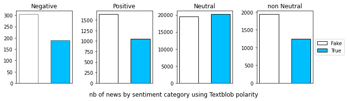
There are more positive and negative news (considering the overall sentiment of a news, the polarity!) among the Fake news then among the True news. The fourth plot confirms that the Fake news are more sentimental than the True news that tend to be more neutral.
Interpretation
As mentioned above, Real news come from a crawler that went through Reuters’ website, thus as expected this type of news aims for high level journalism which implies passing on news in the most authentic thus neutral way. This can be seen in the lack of sentiments and higher neutrality in Real news compared to the Fake ones as we saw in the plots. On the other hand Fake news articles were collected from unreliable websites or personal tweets thus they are more likely to be opinionated or to have a populist tone of voice which is usually discouraged in news articles that should be factual and neutral. The problem of populist articles is that readers can often get distracted by the emotion of the article and skip the verification.
Politeness
To compute the politeness of each news, we used the politeness library which is part of the Stanford Politeness API that was used by the authors. The politeness classifier takes as input a sentence and its parses and returns the politeness of that sentence. The politeness of a news is computed as the average of its sentences politeness’s. To compute the parses, we first relied on the annotate method of the Stanford coreNLP that is computed while computing the sentiments, but as we were forced to stop this method at a certain point, and we had to switch to another method to compute the remaining parses. For this we used TextBlob library that computes the parses in the same way.
We show here the average politeness for the Fake vs True news:
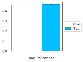
The average politeness of the Fake and True news are very close and the std is very small. We performed a statistical test and found that the difference between the mean politeness of the Fake and Real news is significant.
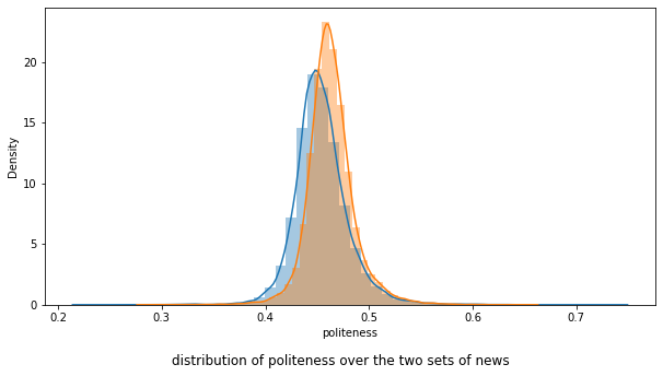
We visualize here the distribution of the politeness for the two sets.
Interpretation
The small difference between the politeness of the True and Fake news, can be due to the fact that Fake news, like in tweets, can sometimes get personal and thus less polite.
Talkativeness
We computed the talkativeness of each news, which consists of the number of sentences and the number of words per news. Here also we started with the CoreNLP annotate method then switched to other methods form the NLTK library. We show here the average talkativeness for the Fake vs True news:
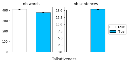
There is a significant difference in the average number of words between the two sets, with the Fake news having a higher value on average with a very small std for both sets. However, for the number of sentences, we can see from the plot that the average values are very close. We performed a statistical test on the number of sentences and found that the p_value is not significant thus we cannot conclude on the difference.
Discourse connectors
We were not able to reproduce the same work done by the authors to extract the discourse connectors due to the lack of information. Thus, we made our researches on the internet to either find predefined methods that do the task or collect the different markers for the feature and compute the number of their occurrences in the news.
-
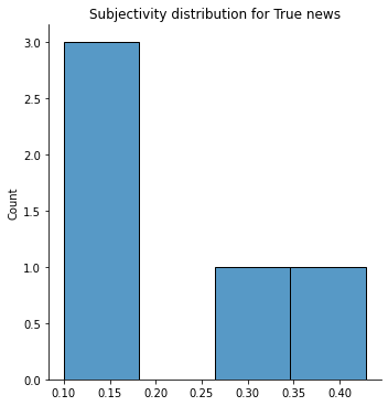
Subjectivity
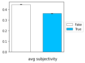
for the subjectivity we used a predefined method from TextBlob library that computes it for a given text. It returns a float in the range [0.0, 1.0] where 0.0 is very objective and 1.0 is very subjective. we show here the results we got for the average subjectivity for the Fake and Real news:
Interpretation
The Fake news are on average more subjective than the True news, with a small std. This is explained by the fact that subjectivity variates inversely to neutrality, thus in Fake news we have given the populist tone we tend to use strong words like ‘resounding’ and ‘astonishing’.
-
Expansion, contingency and comparison
For these features, no predefined method was found. Thus, we collected markers from the internet for each of them and combined them with the features that we extracted from the diplomacy dataset, to get the most complete set of markers. we show here the results we got for the average values of the expansion, contingency and comparison features for the Fake and Real news:
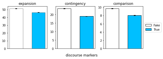
On average Fake news contain more expansion, contingency and comparison discourse connectors than the True news, with small standard deviations. This shows that True news are less eloquent than Fake news. Short sentences strait to the point are factual whereas long sentences that compose Fake news need more discourse connectors.
-
Premises and conclusions
There was no predefined method for this feature as well. We collected the markers from the internet and combined them with the features that we extracted from the diplomacy dataset, to get the complete set of markers.
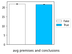
the average number of premises and conclusions for the Fake and True sets are close, with small std. We performed a statistical test and found a non-significant p_value thus we cannot conclude about the difference.
Classification with MLP (Multi-Layer Perceptron)
After extracting and analyzing these features, we built an MLP model that classifies the Fake and True news using them. The objective here is to verify if the “Linguistic harbingers of betrayal” methods generalize to other datasets. We only retain the features that have been computed for all the dataset and that have been used by the authors for homogeneity to train our model. We thus used only the following features: nb_sentences, nb_words, politeness, premises_conclusions, subjectivity, polarity, comparison, contingency and expansion. To train the model we gave labels to distinguish the two datasets, 1 for the True news and 0 for the Fake news. We normalized the data with the z_score scaling and we split it randomly into 80% of train set and 20% of test set.
Model architecture:
We build a model with:
- 15 neurons as input layer
- 256 neurons for the first hidden layer
- 64 neurons for the second hidden layer
- 1 neuron for the last layer that is going to provide the output
- We add early stopping and L2 regularization to avoid overfitting
The model achieved an Accuracy of 0.826 on the test set.
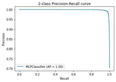
We present here the precison_recall curve of our model:
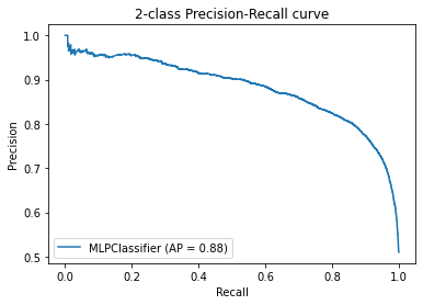
The Precision-Recall curves summarize the trade-off between the true positive rate and the positive predictive value for a predictive model using different probability thresholds. We see that the model performs well as we got an average precision of 87% and it has a considerable AUC (Area Under the Curve).
As we can see the model performs pretty well with those features, which might imply that they generalize well for these kinds of analogous NLP classification problems.
From the performance of this model, we can conclude that these features are strongly correlated to weather news are Fake or not.
Now we will train new models on the ‘text’ of the two datasets using standard deep learning and NLP techniques. The goal here is to give the model the freedom of learning its own features and then compare them with the ones of the authors and see how good they are at classifying news.
Textual analysis
Visualization
We started by visualizing some textual properties of our dataset to get some insights.
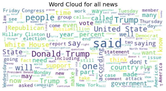
Here we see the word clouds that we generated for all the news:
And here we plot the top 10 n_grams of sizes 1, 2 and 3:
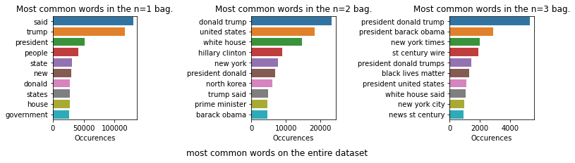
We can see through these plots that ‘said’ is one of the most common words in both datasets, thus the dataset is comprised of a lot of quotes or hearsays about various eminent political figures (Trump, Obama, Clinton, rex tillerson …) and their political parties (Republican or Democrat). The dataset also quotes various infamous news sources (Fox news, New York Times, …). We see also a lot of recently trending topics in the world like “Black lives matter”. Central hubs of power are (New York , North Korea, the White House) are also mentioned all the way throughout the news. Thus, the lingo is mostly based on US political news (internal or external).
After these visualizations, we developed two models to classify our data. The first is an MLP model combined with TF-IDF while the second is a more complex one, an RNN model. We describe in the following sections these two models and their results.
Classification with MLP (Multi-Layer Perceptron)
To approach this classification problem we first want to create a vector space for our documents. We opt for the TF-IDF vectorizer to map our documents to vectors who have as features the TF-IDF value of the most common set of words in the different news articles. We got 2860 words which are the words that are present in at least 1% of the documents. The choice of an MLP came naturally as it’s extremely performant to approximate complex multivariate mappings in higher dimensional spaces. Before training, we normalized the datasets using the L2 norm. We then split the data randomly into 75% of train set and 25% of test set.
Model architecture:
We build a model with:
- 2860 neurons as input layer
- 300 neurons for the first hidden layer
- 100 neurons for the second hidden layer
- 50 neurons for the third hidden layer
- 1 neuron for the last layer that is going to provide the output
- We add early stopping and L2 regularization to avoid overfitting
The model gave an Accuracy of 0.986, on the test set.
We present here the precison_recall curve of our model:
We see that the model performs extremely well as we got an average precision of 100% and it has an almost perfect AUC (Area Under the Curve).
Here we analyze how the MLP classifies the news.
We inspect the subjectivity of the words having a higher likelihood of beeing classified as Fake or True, respectively.
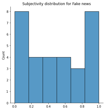
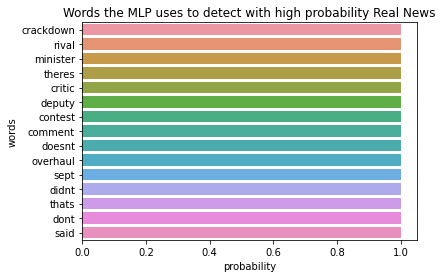
We can clearly see that the words with a higher likelihood to be classified as Fake have no correlation with the subjectivity feature. This implies that the model found its own decision boundary for classification, which is a small subset of the combination of certain features with certain values. The model does not implicitly pick up the features defined in the previous sections. This is quite common with MLP models as they are good at finding implicit decision boundaries while us as humans have more explicit decision boundaries for this kind of problems.
But !
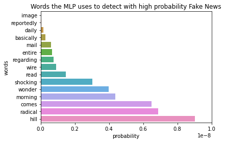
The MLP model learned through training words that are the most common on each dataset and uses them to classify the new news it gets. Thus, if we compose a sentence containing some of the most common words of the Fake dataset, we are almost sure that the model will classify it as Fake. The MLP classifier, thus has a bias towards certain words being used in this context. This is something that the previous analysis (with sentiments) clearly does not have a bias towards these words because it operates at a certain level of abstraction above: only the feeling that comes out of the sentence in general is taken into account.
We present here an example of a Fake statement that we fed to the model to see how it classifies it. The sentence contains two of the words the MLP uses to detect with high probability Real news, which is ‘said’, ‘deputy’.
print("probability of classifying the sentence as true is: ", clf.predict_proba(vectorizer.transform(["The deputy said that the WAP group is the best"]))[0][1])
probability of classifying the sentence as true is: 0.9999736807309447 ![]()
RNN (Recurrent Neural Network)
The problem with the MLP with the TF_IDF model is that it does not take into account the structure of the text, its length or the order of the words in that text. This can be an important feature in texts especially in the English language that is very sensitive to the order of the words in a sentence. Thus, if we want to take it into account, we should change the way we approach this problem. In fact, a text can be seen as a series of words, thus an RNN (a perfectly fitted model for time series) can be good to classify these news.
Not all texts have the same length, and since the RNN model requires inputs of the same size, we will pad the text and we set them all to a length of 270 words.
We implemented an RNN model using LSTM layers. LSTM (long short term memory) because sequences are kind off long (270 times steps!) thus we need the forget gate to be able to remember previously seen inputs and thus its decisions are influenced by what it has learnt from the previous time steps, that’s what makes RNNs more powerful than the other models for this kind of classification. We split the data randomly into 75% of train set and 25% of test set.
Embeddings
Some words often come in pairs, like nice and easy or pros and cons. So, the co-occurrence of words in a corpus can teach us something about its meaning.
Sometimes, it means they are similar or sometimes it means they are opposite.
The point from embeddings is it to create a vector such as: if two words are similar, they should have similar values in this projected vector space.
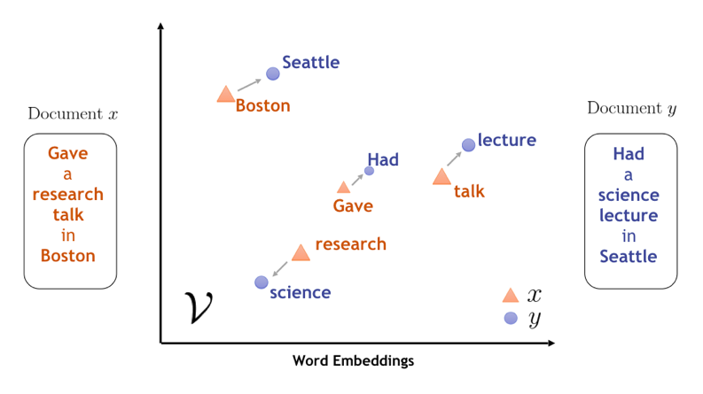
In our case, we use GloVe, which is an unsupervised learning algorithm for obtaining vector representations for words. Training is performed on aggregated global word-word co-occurrence statistics from a corpus, and the resulting representations showcase very powerful linear substructures of the word vector space.
More precisely, we use pre-trained word vectors from twitter with 2B tweets, 27B tokens, 1.2M vocab, uncased.
We opt for 50 dimension version (as it is enough for our project).
To note how important the embeddings are the model initially was run without them and only reached 82% accuracy at best and 70% F1 score on the training set with very slow convergence (after 100 epochs, which was almost 1 hour of running with the Google Colab with GPU). However, stay tuned to see what is the effect of adding an embedding layer to the model ![]()
Model architecture:
We build a model with:
- embedding layer that takes an input of 270 entries vector and outputs a 270 time steps each with a vector of size 50
- bidirectional LSTM layer that outputs a vector of size 64
- dense layer of 64 neurons
- dropout layer of 0.2
- 1 neuron for the last layer that is going to provide the output
- We add early stopping, learning rate reducer and Elastic net regularization to avoid overfitting
Tadaaa!!! The model gave an accuracy of 0.992 on the test set and 0.992 for the F1 score!
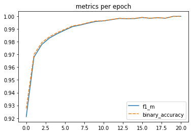
The model performs extremely well with very fast convergence (on average less than 10 epochs) as seen in the graph.
We also check if the problem has the previously mentioned bias to words highly associated to fake news. We use the same previous sentence and we feed it the classifier.
sad_us_rnn = pad_sequences(tokenizer.texts_to_sequences(["The deputy said that the WAP group is the best"]), maxlen = 270, padding='post', truncating='post')
print("probability of classifying the sentence as true is: ", model.predict(sad_us_rnn)[0][0])
probability of classifying the sentence as true is: 0.0012544087 ![]()
So !
As we can see, given that this model does not rely on individual words but rather the entire structure of the sentence/text, it managed to actually bypass the bias that the MLP was unable to.
Conclusion
As we saw throughout our project, the features that the authors used to detect betrayal in the diplomacy game are pretty generenic, in a sense that it generalizes pretty well to completely different yet analgous NLP classification problems (for example the Fake and True news dataset). We also ran two different models, an MLP model and a RNN model on the texts of our second dataset and got pretty good results. However, these trained models do not generalize well when they will be tested on other sets of news like for example news from the Asian news. This is due to the fact that these models learned word specific features from the training sets and those features do not work well with new different sets.
Although not as efficient, the features that the author used generalize better because they are not specific to some type of datasets, but rather specific to a communication intention (lying, betraying, spreading rumors) and how us as humans have a tendency to react when we are confronted or we doing these actions. And thus is on a hugher level of abstraction.
Authors
Zeineb Ayadi
Nizar Ghandri
Ana Lucia Carrizo Delgado
References
- https://stanfordnlp.github.io/CoreNLP/
- https://towardsdatascience.com/recurrent-neural-networks-d4642c9bc7ce
- https://nlp.stanford.edu/projects/glove/
- https://textblob.readthedocs.io/en/dev/
- https://vene.ro/betrayal/
- https://cran.r-project.org/web/packages/politeness/vignettes/politeness.html